Signal Intelligence - Where the magic happens

The purpose of this post is to begin with an unknown signal and identify its main characteristics. Along the way, we will likely consider and discard various hypothesis, ultimately focusing on a specific type of signal.

Disclaimer: This is not meant to be a comprehensive guide on working with all types of signals, but rather to provide an understanding of the necessary process to deal with them.

I will start from a given IQ from which we only know that the samples are record in C32 format. I do not have information about the sample rate, modulation, or any other characteristic of the signal. So, we will start by assuming some details to be able to begin working. (We are currently working on a detailed post about IQ format)

• In this opportunity we are going to use the following tools:
  • GNU Radio (companion)
  • python
    • numpy
    • pylab or matplotlib

As we are working in the digital domain, after the ADC, there is no need to know the "real physical" sample rate. Instead symbol rate, we can work with "samples per symbol".

Ok, lets start now, first step is to Inspect the File, in my case I have this IQ as an example :

• # 1: Inspect the file

  • There are several options to choose. If you have the opportunity I will encourage you to use all of them.

  • ## Option A

    • In a python interpreter (I use IPython) you can copy the following lines:

    • import numpy as np
      import pylab
      signal = np.fromfile("example.iq", dtype=np.complex64)
      length = len(signal)
      # Plot in time domain 
      # a few samples
      half_length = length/2
      pylab.plot(signal[:int(half_length)]); pylab.grid(); pylab.show()
      # Plot in frequency domain
      # Fs = sample rate
      pylab.specgram(signal[:int(half_length)], Fs=1); pylab.show()
      

    • With these lines, you will be able to understand the length of your file and plot it in the time and frequency domains.

    • If the file is too big or your computer does not have enough resources the plot might take a while to load. Therefore, I recommend plotting only slices of the signal. In this case, we plotted only half of it. (You will need to plot the second half after that, or you can take the risk and plot the entire signal at once.)

    • It's important to mention that in both plots, we have multiple arguments to use. This allows us to see the signal in different ways and focus on the things we care about.

      • For example, the pylab.specgram function receives, as an argument, the size of the window over which the FFT is being calculated(NFFT = <windows_size>). As you may know, there is a trade-off between temporal and frequency resolution directly related with the window length. A shorter window allows for better temporal resolution but worse frequency resolution.

    • Personal appreciation: I have been using inspectrum to do the specgram plot and it is really useful and easy to use (and you do not have to worry for your computer resources to support the file).

  • ## Option B

    • GNU Radio is one of the most widely chosen applications in the telecommunications world. It is really useful for working with a signal. I am leaving here the flowgraph used in this case.

    • This is a really simple flowgraph, only a couple of blocks are involve:

      • the file source where you need to add the Iq to be used as a source. Here is important to configure it in "repeat" mode so it is always transmitting the signal.
      • the Throtleis the block in charge of handle the speed of the flowgraph. If you do not include it, gnu radio will try to run the flowgraph at the max speed of your computer and it probably consume all your resources.
      • Finally, the blocks you use to see the signal. In this case, we are using:
        • QT GUI Frequency Sink
        • QT GUI Time Sink
        • QT GUI Waterfall Sink As in the other blocks, there are a lot of variables than can be configured to improve an make the plot look pretty. I would leave this up to you, but just as a recommendation it is always a good idea to enable the control panelso you can interact with the signal in realtime.

      It's important to note that the GUI plots in GNU Radio may experience some sample losses, which means you might miss critical information in your signal. This issue can occur if you're using a high sample rate and your signal packets are very small. A tool to mitigate this and plot the signal in real time is fosphor.

  • OPTION A or OPTION B will allow you to see something like this:

    • ### Frequency Domain

      -

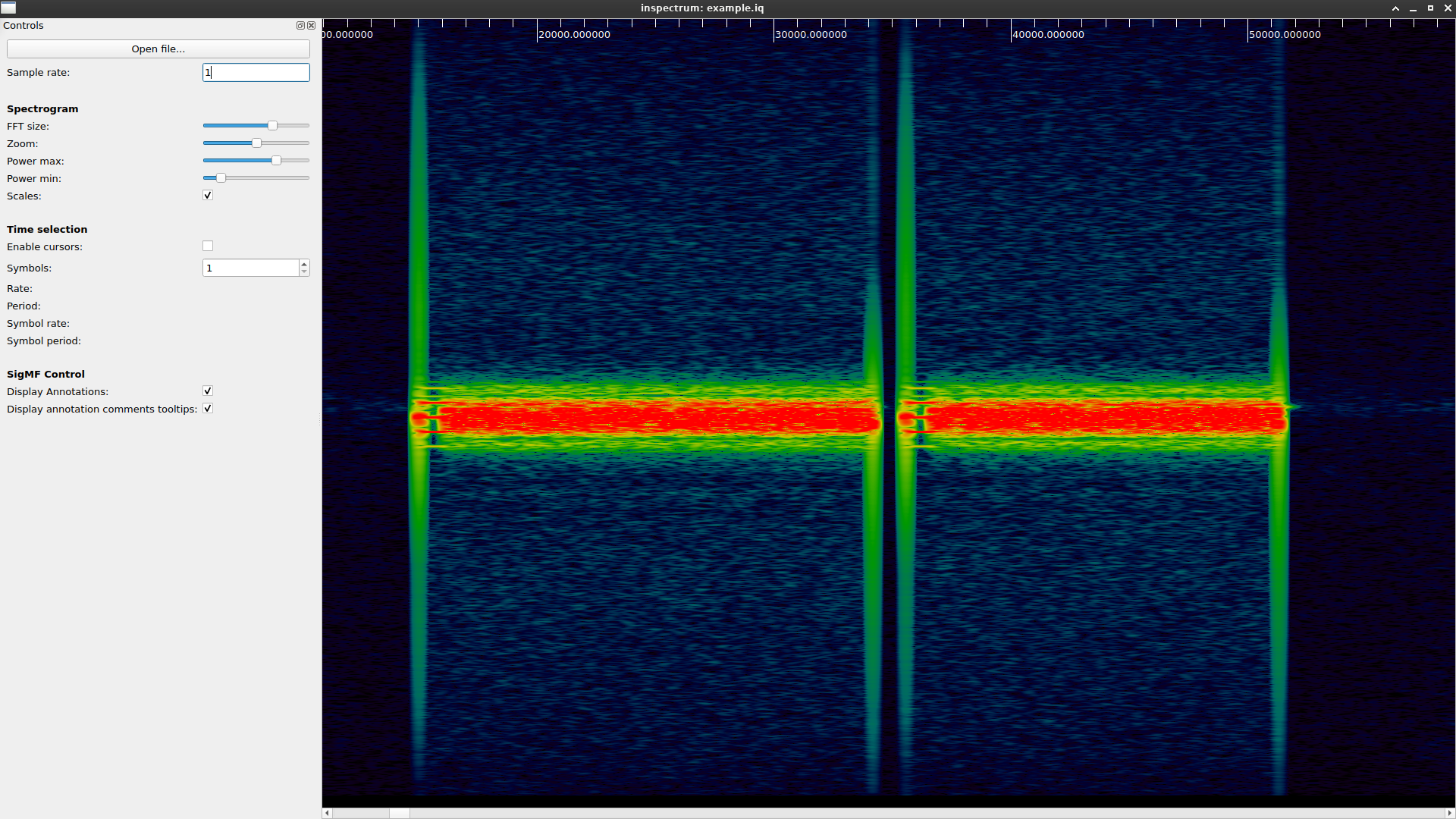
      • It is possible to see some differences, depending on the FFT size.
      • In the picture it is easy to identify areas where there is energy and areas where there is not. This gives us the first clue about our IQ. It seems that we are working with a packetized communication. By visual inspection we can find the beginning and end of each packet, and therefore, count the amount of packets we have in the signal (in this case we have 4 packets.)

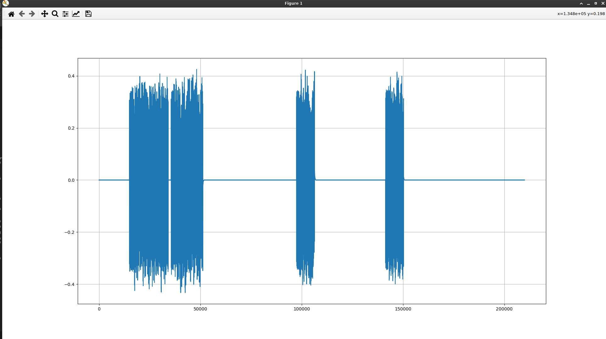
    • ### Time Domain

      • 
      • This plot confirm what we were seeing in the Frequency domain.
      • Since we were able to identify the packets, we can cut only one of them to work in the next steps. For example, using the last image as a reference, we can manually detect the beginning and the end of one packet.
      • To save it as a new file, we can use the following line :

      signal[int(1.4e5):int(1.52e5)].tofile("example_one_pkt.iq")

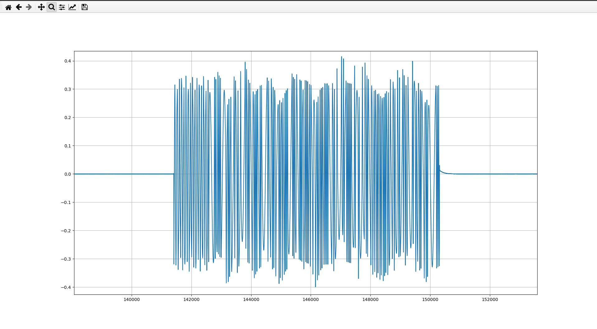
      - I ended up having something like this ![python_plot_one_pkt](python_plot_one_pkt.png)
      - This last image reveals some information about the signal we are working with. The amplitude of the signal remains constants throughout the entire duration of the packet, so we can discard the possibility of an AM modulation (including PAM, QAM, etc).
      
      
      

    Lets now plot the packet using specgramand playing with the windows size:

    • Small Window size:

      pylab.specgram(signal[int(1.4e5):int(1.52e5)], Fs=1, noverlap=32, NFFT=64)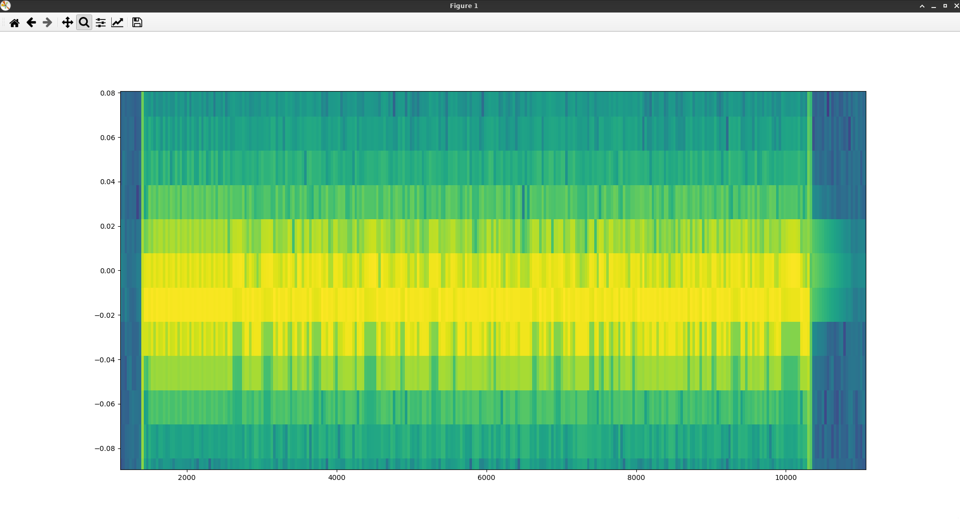

      This image is pretty useful to understand the modulation of the signal we have. If we observe the plot we can see that for every point in time (horizontal axis) there is a different value of frequency (vertical axis). This particular pattern indicate that the signal is being shifted in frequency over the time, meaning that we are working with a FSK modulated signal.

    • Big Window size:

      I will stick with inspectrum plot in this case as it let you play with the colours to have a better appreciation of the signal.

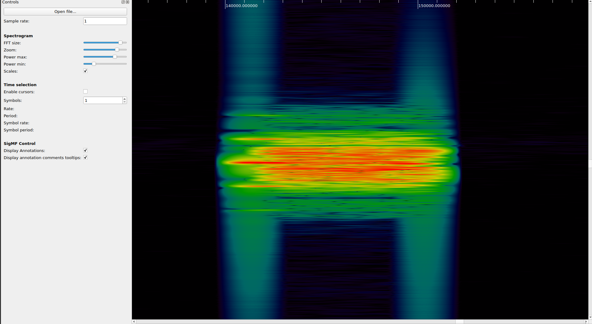
      Here it is also possible to identify another characteristic of a FSK signal. In this case, we can see the 2 carrier signals, each of them separated the same distance from the center carrier. Measuring the distance from the carrier signal to the center we can have a first idea of the deviation used by the modulator.

Recap: Up to now, we know that we are working with a packetized communication and that the signal is FSK modulated.

Next step, could be to find the samples per symbol or SPS relation. Where:

SPS = symbol rate / sample rate

There are couples of way to find it, but lets go with the easiest and simpler one just to have an approximated idea.

Lets use the QT GUI Frequency Sink from GNU Radio. (you can use the same flowgraph showed before but just leaving this particular sink)

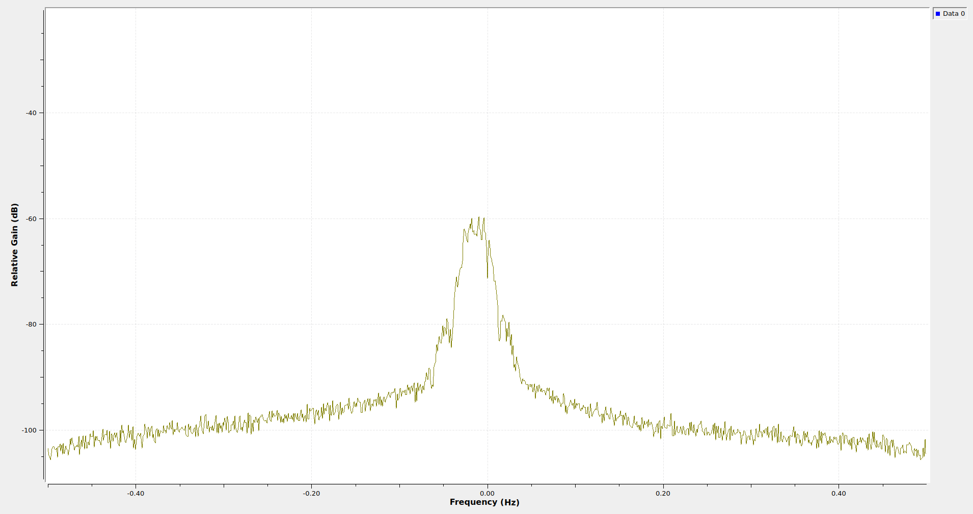
We can do a visual inspection of the this plot and try to estimate how much of the spectrum is being used by our signal. It is not easy to find a exact value but doing an approximation we can say that the signal goes from -0.06Hzto 0.04Hz so it occupies around 0.10Hzof an spectrum of 1Hz. This is the same of saying that:

bandwidth = symbol rate = 1/10 and therefore : SPS = 10

Ok, we have a possible value for the SPS but we can´t guarantee that is the correct one. Moreover, I am pretty sure that it is not correct because in our assumption we are not considering the deviation that the modulation could have. To be closer to the right value we should consider Carson's Rule and it is a bit more complicated.

I prefer to go in another direction. So what we can do now, is try to demodulate the signal and see what we find.

• # 4: Demodulate the signal (using GNU Radio )

  I have prepared a new GNU Radio flowgraph for this part.

  • We are working with a FSK modulation. One way to work with the signal is to use a quadrature demodulator . The input of this block needs to be complex baseband and the output is the signal frequency in relation to the sample rate, multiplied with the gain. Mathematically, this block calculates the product of the one-sample delayed input and the conjugate undelayed signal, and then calculates the argument of the resulting complex number

  • On the other hand we use a complex to magblock that allow us to know the power of the signal. It is possible that the amplitude of the signal is not enough to be recognized in the plot, so we can use a multiply constjust to make it easier to see.

  • The number of points in the QT gui Time Sinkneeds to be configure to allow us to see the entire signal in the plot. You can use the control panel to adapt it in a more interactive way.

    • activate Control Panel
    • use +X to increment the X Max
    • set up normal normal trigger
    • Stop the signal while you see a packet in the screen.

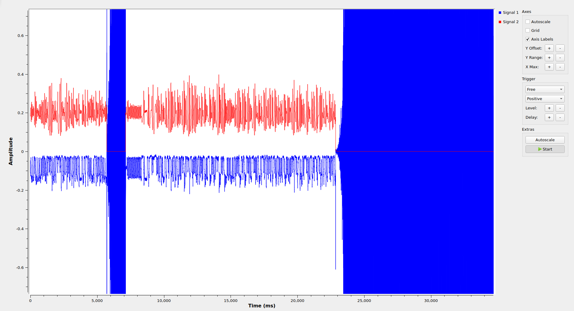
  • The result should be something like this:

  • The red line (output of the complex to mag block) help us to quickly differentiate between the signal and the noise . The last part of the plot (red line = 0) is noise, while the parts where red line > 0 are the packets present on the signal. I leave it to the reader, the task of understanding why the output of the quadrature demodulator amplifies the noise and attenuate the signal. We will explain more about this topic in a future post.

  • At this point we pretty much have all the information of the signal, we should even be able to identify all the bits that are present in it.

  Disclaimer: depending on the SNR of your file, you may not be able to see the signal as clearly as it can be seen in this example. In that case, it might be helpful to add a Low Pass Filter block to the flowgraph (in the previous step we saw the bandwidth of the signal, so the only thing to consider is that the cutoffshould include it.)

  • As it is possible to identify the bits of the packet, you can (it is not a easy job) count the bits and try to understand the message. To be honest, I do not think this is something that would lead us to any significant point, in most of the cases the packets are randomized or even encrypted, so I would not expect to find much. What we can do, and it should be much easier, is try to find some pattern, for example is pretty common to have a known preamble at the begging of each packet for the radio to recognize them. In fact, if we take a deeper look at the last plot, we can see something like this at the beginning:

  

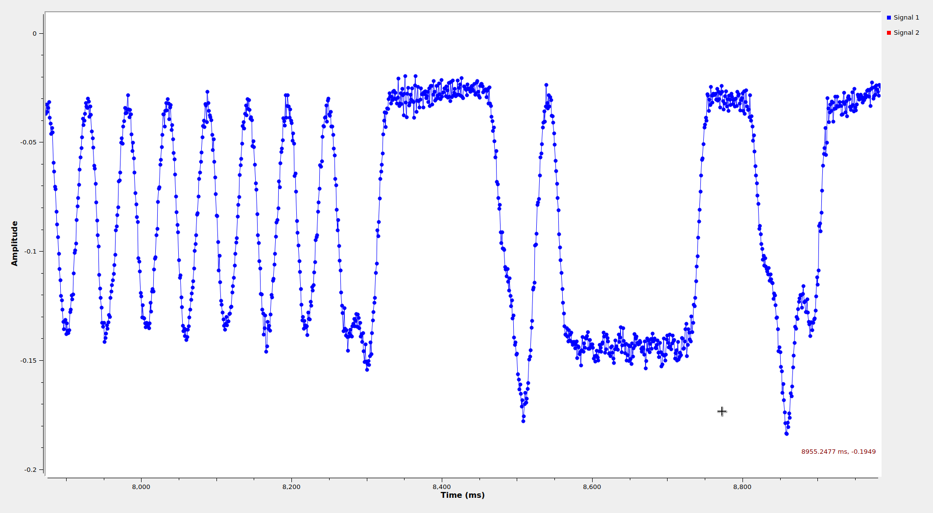
  It is pretty clear that the signal start with a repetition of 01010101. This sequence is one of the most used one, in hex it can be translate as 0x55 or 0xAA.

  I also took the opportunity to add to the plot, the dots that can bee seen in the last image (you can also add them with "center button of the mouse" --> "signal 1" --> "Line Marker" --> "circles"). This dots, show the amount of samples that we have in our signal. So if we cut only one symbol and count the dot we will find the Sample per symbols relation.

  In this case SPS = 26

  This value is again an approximation (much closer than the previous one) and should not be consider as the final value. Also, as in this case it is pretty big, it is difficult to count. To mitigate this, it is possible to do a fractional resamplerand reduce the amount of dots to make it easier (do it with care to avoid breaking the signal).

At this point, we have already learned how to detect the packet and how to identify the bytes, so we can say that our objective was accomplished. A new post on how to decode a packet will be release soon to continue with the last steps. In the meantime I will recommend you to take a look in gr-satellites repository, if you have luck you will find the path already solved there.